Programming-assignment: Illustrating problems in the adjustment of covariates when doing causal inference

Authors: Patricia Fernandez Moreno, Sofía González Matatoros, Víctor Manuel López Molina and Álvaro Pita Ramírez

1. Introduction to causal inference

According to the Encyclopedia Britannica (2022), induction is a means of reasoning from particulars to generals and one example of this is causal inference. The objective of this process is to infer the actual effect of a particular element within a more complex system, considering the global outcome under changing conditions (Pearl & Judea, 2009). At this point, it is important to clarify that association does not imply causation, in other words, two elements can be related because they belong to the same interacting network, but its relationship cannot be due to a cause-effect process.

Back to the initial topic, when we want to make an interpretation of the statistical results in this type of scenarios, a relevant aspect is to choose on which covariates we are going to adjust in the analysis. Therefore, the aim of this report is to explain which are the consequences of doing an incorrect analysis, since we are aware that the process of causal inference is highly used in biomedical research.

2. Explaining our DAG

To illustrate how to perform the correct analysis, we are going to examinate the following scenario described on this code

library(dagitty)
if(!suppressWarnings(require("rethinking", quietly = TRUE))) {
  drawdag <- plot
} 

dag1 <- dagitty("dag {
W -> X
W -> Y
X -> Z
Y -> Z
e_x -> X
e_y -> Y
e_zx -> Z
e_zy -> Z
}")

coordinates(dag1) <- list(x = c(W = 2.5, X = 2, Y = 3, Z = 2.5, e_x = 1.5, 
                                e_y = 3.5, e_zx =1.5, e_zy = 3.5),
                          y = c(W = -0.5, X = 0, Y = 0, Z = 0.5, e_x = -.25, 
                                e_y = -0.25, e_zx = .5, e_zy = .5))
## plot(dag1)
drawdag(dag1)
drawdag(dag1, xlim = c(-2, 2), ylim = c(-2, 3)

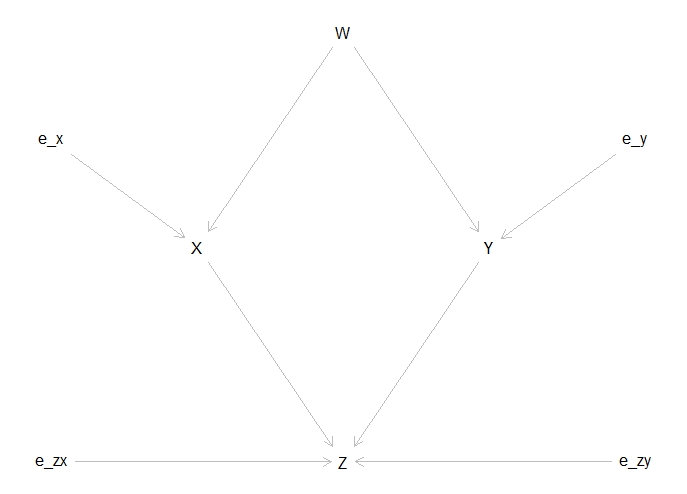
Considering this DAG, we can make these observations

• X and Y are associated throw W, which is a cofounder, so conditioning on W would render them independent.
• Z is a collider, depending on X and Y.

3. Choosing covariates

3.1. Example with multiple regression

Given the diagram explained above, we are going to check whether the effect of X and Y over Z is better predicted by fitting or not by the cofounder W. To this end, we will execute the function dist_multiple() described in the following box

dist_multiple <- function(N = 50, b_xw = 3, b_yw = 2, b_zy = 5, b_zx = 4, 
                            sd_x = 1, sd_y = 5, sd_z = 2, B = 2000, w_min = 1, 
                            w_max = 5) {
  
  X_no_W <- rep(NA, B) 
  # we initialize the list with the coeficents of Z when the model is 
  # not adjusted
  X_yes_W <- rep(NA, B) 
  # we initialize the list of p-values the coeficents of Z when the model is 
  # not adjusted
  pv_X_no_W <- rep(NA, B) 
  # we initialize the list with the coeficents of Z when the model is adjusted
  pv_X_yes_W <- rep(NA, B) 
  # we initialize the list of p-values the coeficents of Z when the model is
  # adjusted
  
  for(i in 1:B) { 
    W <- runif(N, w_min, w_max) # The variable W follows an uniform distribution
    X <- b_xw * W + rnorm(N, 0, sd = sd_x) 
    # The variable X follows a normal distribution, influenced by W
    Y <- b_yw * W + rnorm(N, 0, sd = sd_y) 
    # The variable Y follows a normal distribution, influenced by W
    Z <- b_zy * Y + b_zx * X + rnorm(N, 0, sd = sd_z)
    # The variable Z follows a normal distribution, 
    # acting as a collider of X and Y
    
    m1 <- lm(Z ~ (X + Y)) 
    # linear regression of Z depending on X and Y without adjusting
    m2 <- lm(Z ~ (X + Y) + W) 
    # linear regression of Z depending on X and Y adjusting by W
    
    X_no_W[i] <- coefficients(m1)["X"] 
    #estimated coefficient of the effect in model m1
    X_yes_W[i] <- coefficients(m2)["X"] 
    #estimated coefficient of the effect in model m1
    
    pv_X_no_W[i] <- summary(m1)$coefficients["X", "Pr(>|t|)"] 
    #p-value in model m1
    pv_X_yes_W[i] <- summary(m2)$coefficients["X", "Pr(>|t|)"] 
    #p-value in model m2
    
    rm(Z, X, Y, W) # We prepare the variables for the next call of the function
  }
  cat("\n Summary effect without W\n")
  print(summary(X_no_W)) #summary of the coefficents without adjust by W
  cat("\n s.d. estimate = ", sd(X_no_W)) #standard deviation without adjustment
  cat("\n\n Summary effect with W\n")
  print(summary(X_yes_W)) #summary of the coefficents without adjust by W
  cat("\n s.d. estimate = ", sd(X_yes_W), "\n") 
  #standard deviation with adjustment
  
  op <- par(mfrow = c(2, 2))
  hist(X_no_W, main = "Effect without W in the model", xlab = "Estimate")
  abline(v = b_zx, lty = 2)
  # histogram of the unadjusted coefficents
  hist(X_yes_W, main = "Effect with W in the model", xlab = "Estimate") 
  abline(v = b_zx, lty = 2)
  # histogram of the adjusted coefficents
  
  hist(pv_X_no_W, main = "Effect without W in the model", xlab = "p-value") 
  # histogram of the unadjusted p-values.
  hist(pv_X_yes_W, main = "Effect with W in the model", xlab = "p-value") 
  # histogram of the adjusted p-values.
  par(op)
}

When we call the function dist_multiple(), the following output is:

Summary Effect without W

Min.	1st Qu.	Median	Mean	3rd Qu.	Max.
3.688	3.944	4.001	3.999	4.057	4.382

s.d. estimate = 0.0866533

Summary Effect with W

Min.	1st Qu.	Median	Mean	3rd Qu.	Max.
2.878	3.811	4.002	4.003	4.203	5.410

s.d. estimate = 0.2954924

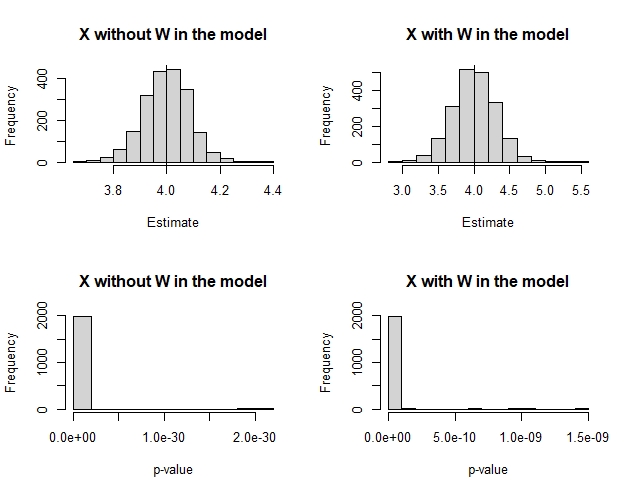
It is observed that when adjusting for W the standard deviation increases 0.11 units, while the mean hardly differs. Therefore, in this case adjusting for the covariate W is a bad idea, because it renders X and Y independent, affecting the analysis.

3.1. Example with simple regression

In this section we will try to find out the individual effect exerted by X on Z. To this end, we will apply the function dist_simple, to see which scenario provides the correct analysis. Here we have four options for adjusting: none, W, Y, or W and Y.

dist_simple <- function(N = 50, b_xw = 3, b_yw = 2, b_zy = 5, b_zx = 4, 
                        sd_x = 1, sd_y = 5, sd_z = 2, B = 2000, w_min = 1, 
                        w_max = 5) {
  X_no_W <- rep(NA, B) 
  X_yes_W <- rep(NA, B)
  X_yes_Y <- rep(NA, B)
  X_yes_WY <- rep(NA, B)
  pv_X_no_W <- rep(NA, B) 
  pv_X_yes_W <- rep(NA, B)
  pv_X_yes_Y <- rep(NA, B)
  pv_X_yes_WY <- rep(NA, B)

  
  for(i in 1:B) { 
    W <- runif(N, w_min, w_max)
    X <- b_xw * W + rnorm(N, 0, sd = sd_x)
    Y <- b_yw * W + rnorm(N, 0, sd = sd_y)
    Z <- b_zy * Y + b_zx * X + rnorm(N, 0, sd = sd_z)
    
    m1 <- lm(Z ~ X) # linear regression of Z depending on X (unadjusted)
    m2 <- lm(Z ~ X + W) # adjusted by W
    m3 <- lm(Z ~ X + W + Y) # adjusted by W and Y
    m4 <- lm(Z ~ X + Y) # adjusted by Y
    
    X_no_W[i] <- coefficients(m1)["X"] 
    X_yes_W[i] <- coefficients(m2)["X"] 
    X_yes_WY[i] <- coefficients(m3)["X"]
    X_yes_Y[i] <- coefficients(m4)["X"]
    
    pv_X_no_W[i] <- summary(m1)$coefficients["X", "Pr(>|t|)"] 
    pv_X_yes_W[i] <- summary(m2)$coefficients["X", "Pr(>|t|)"] 
    pv_X_yes_WY[i] <- summary(m3)$coefficients["X", "Pr(>|t|)"] 
    pv_X_yes_Y[i] <- summary(m4)$coefficients["X", "Pr(>|t|)"] 
    
    rm(Z, X, Y, W)
  }
  cat("\n Summary X without adjusting\n")
  print(summary(X_no_W))
  cat("\n s.d. estimate = ", sd(X_no_W))
  cat("\n\n Summary X with W\n")
  print(summary(X_yes_W))
  cat("\n s.d. estimate = ", sd(X_yes_W), "\n")
  cat("\n\n Summary X with W and Y\n")
  print(summary(X_yes_WY))
  cat("\n s.d. estimate = ", sd(X_yes_WY), "\n")
  cat("\n\n Summary X with Y\n")
  print(summary(X_yes_Y))
  cat("\n s.d. estimate = ", sd(X_yes_Y), "\n")
  
  op <- par(mfrow = c(2, 4))
  hist(X_no_W, main = "X without W and Y in the model", xlab = "Estimate")
  abline(v = b_zx, lty = 2)
  hist(X_yes_W, main = "X with W in the model", xlab = "Estimate") 
  abline(v = b_zx, lty = 2)
  hist(X_yes_WY, main = "X with W and Y in the model", xlab = "Estimate") 
  abline(v = b_zx, lty = 2)
  hist(X_yes_Y, main = "X with Y in the model", xlab = "Estimate") 
  abline(v = b_zx, lty = 2)
  
  hist(pv_X_no_W, main = "X without W and Y in the model", xlab = "p-value")
  hist(pv_X_yes_W, main = "X with W in the model", xlab = "p-value")
  hist(pv_X_yes_WY, main = "X with W and Y in the model", xlab = "p-value")
  hist(pv_X_yes_Y, main = "X with Y in the model", xlab = "p-value")
  par(op)
}

Summary X without adjusting

Min.	1st Qu.	Median	Mean	3rd Qu.	Max.
3.820	6.404	7.098	7.082	7.775	10.655

s.d. estimate = 1.022683

Summary X with W

Min.	1st Qu.	Median	Mean	3rd Qu.	Max.
-10.210	1.508	3.951	3.970	6.333	17.020

s.d. estimate = 3.604197

Summary X with W and Y

Min.	1st Qu.	Median	Mean	3rd Qu.	Max.
3.115	3.798	3.996	3.996	4.198	5.184

s.d. estimate = 0.2931457

Summary X with Y

Min.	1st Qu.	Median	Mean	3rd Qu.	Max.
3.679	3.941	3.999	4.000	4.057	4.365

s.d. estimate = 0.08639647

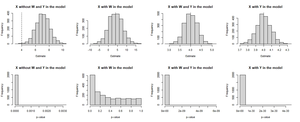
Looking at the results, the mean is found to be closer to reality (mean = 4 and s.d. = 0.086) when adjusting by Y. However, comparing the unadjusted model and the models adjusted for at least one covariate, the latter provide more accurate estimates.

$ Añadir justificación

4. Changing parameters

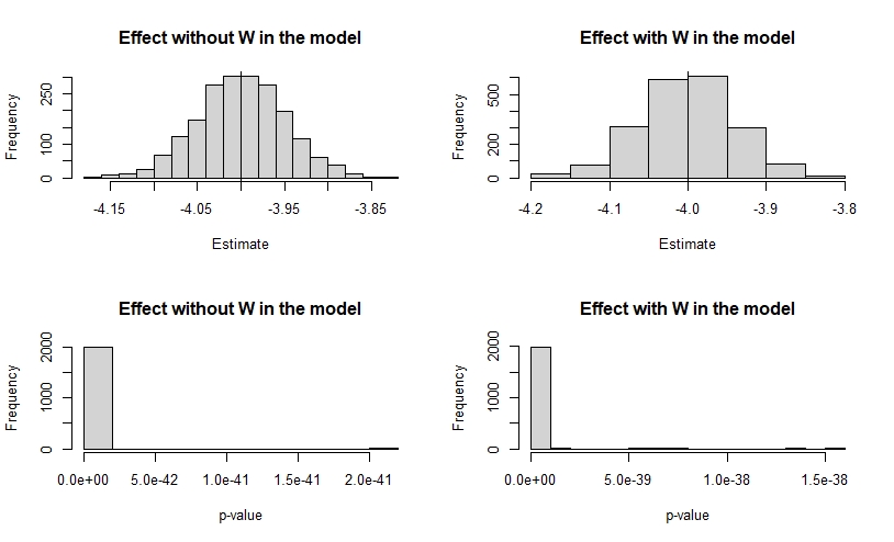
Considering the examples illustrated above, we are going to check what happens if we decrease the coefficient b_zw and its standard deviation calling the functions like this dist_simple(sd_x = 5, b_zx = -4) and dist_multiple(sd_x = 5, b_zx = -4).

4.1. Multiple regression

Summary effect without W

Min.	1st Qu.	Median	Mean	3rd Qu.	Max.
-4.162	-4.034	-3.999	-4.000	-3.966	-3.835

s.d. estimate = 0.05064404

Summary effect with W

Min.	1st Qu.	Median	Mean	3rd Qu.	Max.
-4.191	-4.040	-4.000	-4.000	-3.960	-3.807

s.d. estimate = 0.06008477

4.2. Simple regression

Summary X without adjusting

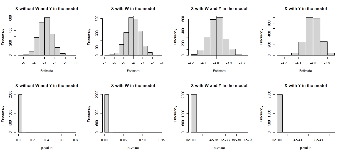
Min.	1st Qu.	Median	Mean	3rd Qu.	Max.
-5.0230	-3.3424	-2.9283	-2.9141	-2.4988	-0.2526

s.d. estimate = 0.6309767

Summary X with W

Min.	1st Qu.	Median	Mean	3rd Qu.	Max.
-6.642	-4.498	-4.009	-4.005	-3.501	-1.280

s.d. estimate = 0.7356117

Summary X with W and Y

Min.	1st Qu.	Median	Mean	3rd Qu.	Max.
-4.189	-4.042	-4.000	-4.000	-3.961	-3.775

s.d. estimate = 0.06130837

Summary X with Y

Min.	1st Qu.	Median	Mean	3rd Qu.	Max.
-4.203	-4.034	-4.000	-4.000	-3.968	-3.855

s.d. estimate = 0.05004781

4.3. Comparison between simple and multiple linear regression

By decreasing the value of the parameter b_zx and increasing the value of sd_x, it is found that the estimates of the deviation of all fitted models improve considerably.

& Añadir justificación

5. Conclusions

Bibliography

Britannica, T. Information Architects of Encyclopaedia. (2022). thought. Encyclopedia Britannica. https://www.britannica.com/facts/thought

Pearl, Judea. (2009). Causal inference in statistics: An overview. Statistics Surveys, 3, 96–146. doi:10.1214/09-SS057.